


Next: 2 Conjugate Gradient Algorithm
Up: 2 Conjugate Gradient Iteration
Previous: 2 Conjugate Gradient Iteration
Contents
Suppose
 is a real symmetric positive definite matrix (so that
 for all non-zero
 ) and consider the function
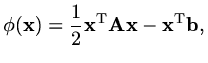 |
(170) |
then
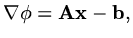 |
(171) |
so that  will be a minimum when
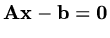 . So to solve the matrix equation
 we can try to find a minimum of the function . We can use this idea to generate an
iterative method to determine an approximate solution of the original matrix equation.
we can try to find a minimum of the function . We can use this idea to generate an
iterative method to determine an approximate solution of the original matrix equation.
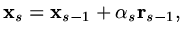
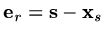
If we have an approximation
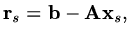
 then the residual,
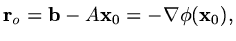 |
(172) |
will give the direction of fastest descent from the curve
 at the point
.
So we can find a value
at the point
.
So we can find a value
 for which
 is smallest.
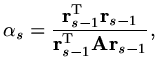
If we solve
is smallest.
If we solve
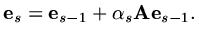
 we obtain
 |
(173) |
so that an iteration algorithm is:
Steepest descents
Choose an initial guess
(e.g.
 ), tolerance
  and calculate
 ,
in
loop for
,
in
loop for
 until
until

This algorithm can converge slowly because it may be repetitively calculating
the same few search directions with only small changes of components in other directions.
Convergence
If the true solution is
 and the error is
 , the iteration formula gives
 |
(174) |
If the eigenvalues and eigenvectors of
are  ,
,
 and the error
is written in terms of
and the error
is written in terms of
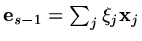 (for some numbers
  ,
leaving out the
,
leaving out the  index),
algebra gives
index),
algebra gives
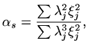 |
(175) |
and we can find the error at the next step. Using a norm
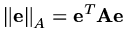 ,
,
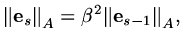 |
(176) |
where
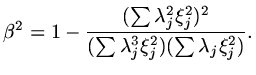 |
(177) |
This formula is not much use without knowing the values of but we can ask
what is the
largest value it can have over all possible combinations of . The method to
answer this question is beyond
this course, but if the condition number of the matrix
is  then
then
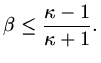 |
(178) |
So convergence becomes slower as the condition number increases but is good if
is less than around 10.
Next: 2 Conjugate Gradient Algorithm
Up: 2 Conjugate Gradient Iteration
Previous: 2 Conjugate Gradient Iteration
Contents
Last changed 2000-11-21