


Next: 3 Multigrid Iteration
Up: 2 Conjugate Gradient Iteration
Previous: 1 Minimisation Problem &
Contents
We will call two vectors
 and
and
 A-conjugate if
 .
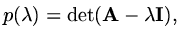
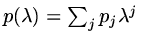
We can also see that if we denote the characteristic polynomial of
.
We can also see that if we denote the characteristic polynomial of
 as
as
 |
(179) |
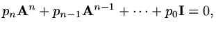
then Cayley-Hamilton's theorem tells us that
 too. If we suppose
 , then
 |
(180) |
and so, as the matrix is non-singular ( ),
),
![$\displaystyle {\rm\bf A}^{-1}=-{1\over p_0}[p_1{\rm\bf I}+p_2{\rm\bf A}+\cdots +p_n{\rm\bf A}^{n-1}]$](img471.png) |
(181) |
and the solution
must be
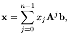 |
(182) |
where
 . Thus the solution is able to be expressed as a linear
combination of vectors of the form
. Thus the solution is able to be expressed as a linear
combination of vectors of the form
 . Let
. Let
 then one approximation strategy
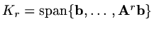
is to try to find approximations from the subspaces
then one approximation strategy
is to try to find approximations from the subspaces
 which successively minimise
  . After
  steps we must have
the solution but of course we hope that when is very large,
we might obtain a good approximation after only a small number of steps.
The obvious way to do this
would be at step
steps we must have
the solution but of course we hope that when is very large,
we might obtain a good approximation after only a small number of steps.
The obvious way to do this
would be at step  , approximating from
  to try to find coefficients
  such
that if
such
that if
 then
then
 is minimised. In this case
 |
(183) |
and so setting the derivatives of with respect to
 to be zero
would mean solving another matrix system of growing size at each iteration.
The idea of conjugate gradient is to find coefficients only once in an expansion
of the solution in terms of a growing set of basis vectors. To do this we need a
different basis for . Suppose we call this basis
to be zero
would mean solving another matrix system of growing size at each iteration.
The idea of conjugate gradient is to find coefficients only once in an expansion
of the solution in terms of a growing set of basis vectors. To do this we need a
different basis for . Suppose we call this basis
 and that the basis vectors are
  -conjugate.
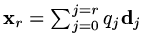
Now if we let
-conjugate.
Now if we let
 then
then
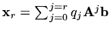
![$\displaystyle \phi (q_0,\ldots ,q_r)=\sum_{j=0}^{j=r}[{1\over 2}q_j^2{\rm\bf d}_j^{T}{\rm\bf A}{\rm\bf d}_j - q_j{\rm\bf d}_j^{T}{\rm\bf b}],$](img486.png) |
(184) |
so now the minimisation problem is almost trivial, each component is independent
of the others and at each step, the existing components do not change. So we only
calculate the components in each direction once.
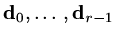
Of course we do have to construct the basis
but since it
has to span and at the  step we already have an -conjugate basis for
  ,
all we have to do is compute one additional basis vector at each step.
,
all we have to do is compute one additional basis vector at each step.
The proof is straight forward. It is almost trivial from our discussion above
that
 |
(185) |
Now
 , so that
 and as
 is A-conjugate with all vectors in , including
 , we must have
 .
.
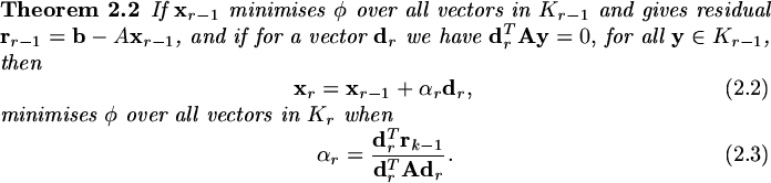
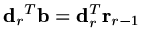
This enables us to carry out one iteration of the Conjugate Gradient algorithm.
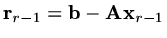
Suppose
 ,
minimises over and the basis vectors
,
minimises over and the basis vectors
 are
-conjugate. Calculate
are
-conjugate. Calculate
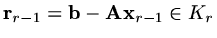 and suppose
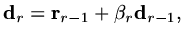 |
(186) |
where  is chosen to make
-conjugate to
is chosen to make
-conjugate to
 ,
,
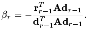 |
(187) |
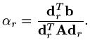
If
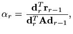 |
(188) |
is a search length, then
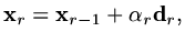 |
(189) |
minimises over and
 |
(190) |
Note that we can also show the
 |
(191) |
and
 |
(192) |
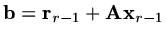
It is worth observing that we only ever need to store four vectors,
 each of which can be replaced as the iteration
proceeds and other than the vector,
each of which can be replaced as the iteration
proceeds and other than the vector,
 there are only inner products to evaluate.
The algorthm is very compact,
there are only inner products to evaluate.
The algorthm is very compact,
Algorithm
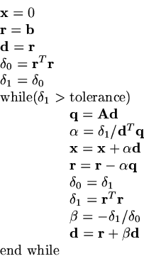 |
(193) |
We do not have time to develop an error analysis but we can note that if the condition
number of the matrix
is  , then the error changes by a factor smaller or
equal to
, then the error changes by a factor smaller or
equal to
 |
(194) |
each iteration. This is considerable better than for steepest descents. Even further
advantage can be gained by preconditioning the matrix
by pre-multiplying the equation
 by an additional matrix. We shall not consider that aspect in this course.
Next: 3 Multigrid Iteration
Up: 2 Conjugate Gradient Iteration
Previous: 1 Minimisation Problem &
Contents
Last changed 2000-11-21