


Next: Acknowedgement
Up: 2 Iterative Methods for
Previous: 2 Conjugate Gradient Algorithm
Contents
Central to a great deal of fluid mechanics is the Poisson equation
 and in two or more dimensions it is common to
obtain approximate solutions by iterative methods.
If we just return to a 1-D model problem,
and in two or more dimensions it is common to
obtain approximate solutions by iterative methods.
If we just return to a 1-D model problem,
 |
(195) |
then for Jacobi iteration
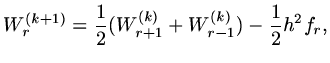 |
(196) |
so that the iteration matrix
 satisfies
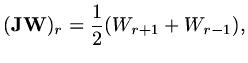 |
(197) |
and if
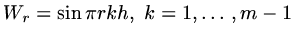 ,
then we see that the eigenvaues of
are just
,
then we see that the eigenvaues of
are just
 and the spectral radius
is
and the spectral radius
is
 so that as the mesh becomes finer, not only are there
more calculations per iteration, the convergence rate becomes poorer. Since
the poor convergence is associated mainly with low frequency errors one way
which has been developed for accelerating
convergence is to carry out some iterations on a coarser mesh where the convergence rate
is better and then to transfer the solution back to the fine mesh.
so that as the mesh becomes finer, not only are there
more calculations per iteration, the convergence rate becomes poorer. Since
the poor convergence is associated mainly with low frequency errors one way
which has been developed for accelerating
convergence is to carry out some iterations on a coarser mesh where the convergence rate
is better and then to transfer the solution back to the fine mesh.
Suppose two vectors are defined,
 which approximates the values
 ,
and
,
and
 with
with
 .
Obviously assume
.
Obviously assume  is even.
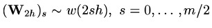
Next define two matrix operators, one which restricts
values on the fine mesh to the coarse mesh, symbolically
is even.
Next define two matrix operators, one which restricts
values on the fine mesh to the coarse mesh, symbolically
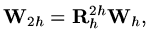 |
(198) |
and an interpolation operator which takes values from the coarse mesh to the fine mesh,
again symbolically
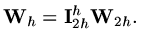 |
(199) |
Multigrid then carries out a number of iterations on the fine mesh, damping out
high frequency errors, transfers values to the coarse mesh and carries out further
iterations on that mesh to damp out low frequency errors before interpolating values back to
the original fine mesh. The overall sequence of iteration on fine mesh, restriction, iteration on
the coarse mesh, interpolation and then further iteration on the fine mesh
represents one cycle of multigrid iteration. In practice a number of meshes are used, not just two.
Symbolically in the case of two meshes,
if we carry out  Jacobi iterations on the fine mesh and
  iterations
on the coarse mesh,
iterations
on the coarse mesh,
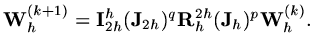 |
(200) |
A key result is that the spectral radius of the iteration matrix can be independent
of  . In practice the finest mesh is chosen with
  and then it is possible to
use up to
and then it is possible to
use up to  meshes, each half the resolution of the previous mesh and a multigrid cycle
is a sequence of (either Jacobi or Gauss-Seidel) iterations on each of the meshes in succession, both after
restricting from fine to coarse, and after interpolating from coarse to fine.
It is also usual to work with residuals, so that if
is our current approximation
and
meshes, each half the resolution of the previous mesh and a multigrid cycle
is a sequence of (either Jacobi or Gauss-Seidel) iterations on each of the meshes in succession, both after
restricting from fine to coarse, and after interpolating from coarse to fine.
It is also usual to work with residuals, so that if
is our current approximation
and
 is a better approximation, then as
![$\displaystyle L_h[{\rm\bf W}_h+\delta {\rm\bf W}_h]={\rm\bf f},$](img530.png) |
(201) |
we have
![$\displaystyle L_h[\delta{\rm\bf W}_h]={\rm\bf f}-L_h{\rm\bf W}_h={\rm\bf r}_h,$](img531.png) |
(202) |
where
 is the residual so that we iterate
on the coarse mesh to solve
is the residual so that we iterate
on the coarse mesh to solve
![$\displaystyle {\rm\bf L}_{2h}[\delta{\rm\bf W}_{2h}]={\rm\bf R}_h^{2h}{\rm\bf r}_h,$](img533.png) |
(203) |
and then
![$\displaystyle {\rm\bf W}_h\leftarrow {\rm\bf W}_h+{\rm\bf I}_{2h}^h[\delta {\rm\bf W}_{2h}].$](img534.png) |
(204) |
Next: Acknowedgement
Up: 2 Iterative Methods for
Previous: 2 Conjugate Gradient Algorithm
Contents
Last changed 2000-11-21