


Next: 2 Fourier Analysis of
Up: 2 Stability
Previous: 2 Stability
Contents
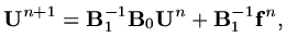
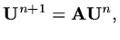
We have seen that time dependent problems are approximated by a vector of values,
 at each time step and further the form of the iteration for these values was
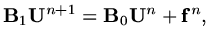 |
(96) |
where
 are matrices. If
 we called the method explicit, otherwise
we referred to an implicit method. If the PDE involved two or more space dimensions, it can
still be dealt with under this framework, elements of vector
we called the method explicit, otherwise
we referred to an implicit method. If the PDE involved two or more space dimensions, it can
still be dealt with under this framework, elements of vector
 have just a more
complicated mapping onto the physical mesh. Thus in principle we have iterations of the
form
have just a more
complicated mapping onto the physical mesh. Thus in principle we have iterations of the
form
 |
(97) |
to calculate the approximation time step by time step. Thus we need first to understand
some things about iterated sequences.
Suppose we have the sequence
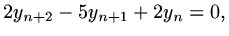 |
(98) |
with  ,
,  .
We look for a solution
.
We look for a solution
 so that
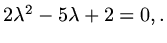 The roots are
 and the general solution
is
and the general solution
is
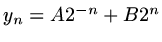 . Using the initial conditions
 |
(99) |
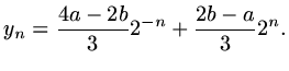
Now suppose we choose the inital values  such that
  , then
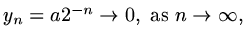 and it might appear that we have a sensible computation to determine
  .
However suppose, because of finite machine accuracy, that
.
However suppose, because of finite machine accuracy, that
 ,
,
 ,
then
,
then
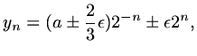 |
(100) |
and for example, if
 (typical single precison accuracy)
then
(typical single precison accuracy)
then
 after only
  iterations! Hence we could not
carry out any practical computations using this iteration without the calulations
being swamped by the growing solution even though the `solution' should have no
component of this mode.
iterations! Hence we could not
carry out any practical computations using this iteration without the calulations
being swamped by the growing solution even though the `solution' should have no
component of this mode.
Consider now a matrix example,
 |
(101) |
where
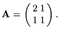 |
(102) |
We look for a solution where
 so that
 , and
, and  is an eigenvalue of
the iteration matrix
is an eigenvalue of
the iteration matrix
 . In this case the eigenvalues are
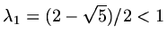 ,
,
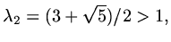 and if we denote
the eigenvectors by
and if we denote
the eigenvectors by
 , the general solution is
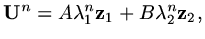 |
(103) |
where  and
and  are constants. Again, if we choose the inital data so that
is zero, machine rounding errors
will still produce a growing component which will swamp the calculation very quickly.
are constants. Again, if we choose the inital data so that
is zero, machine rounding errors
will still produce a growing component which will swamp the calculation very quickly.
Thus one difficulty with calculating iterated sequences is that growing modes lead to
rapid breakdown of a calculation and this `instability' may not be a part of the
original
physical system, but introduced as an artefact of the discretisation of the continuous
system. Often stability is a more challenging practical problem than accuracy.


Next: 2 Fourier Analysis of
Up: 2 Stability
Previous: 2 Stability
Contents
Last changed 2000-11-21