2 Fourier Analysis of Stability

It can be very difficult to calculate all of the eigenvalues of the iteration matrix. One approach which has been very successful in provinding practical stability criteria is to extend the domain of the PDE to the whole real line (or the whole plane ...) and then to look at stability of Fourier modes. On the real line, if $U^n_j$ is assumed to behave like

$$U^n_j\sim [\lambda(k)]^n{\rm e}^{ikjh},$$ (104)

(a discrete analogue of $u(x,t)\sim {\rm e}^{\mu t}{\rm e}^{ikx}$) then we can examine $\max_k\vert\lambda (k)\vert$ to decide on stability of the numerical scheme. It is important to realise that although practical problems do not have infinite domains, they do not have constant coefficients; nevertheless criteria which have come from Fourier analysis of model problems are usually very good predictors for the behaviour of a numerical scheme.

Example 1: Heat Equation

If we have

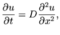$${{\partial u}\over{\partial t}}=D{{\partial^2 u}\over{\partial x^2}},$$ (105)

and we discretise explicitly,

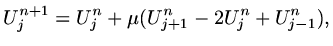$$U^{n+1}_j=U^n_j+\mu (U^n_{j+1}-2U^n_j+U^n_{j-1}),$$ (106)

where $\mu=D\Delta t/h^2$, then substituting the Fourier mode gives

$$\lambda =1-4\mu\sin^2{1\over 2}kh,$$ (107)

so that $\lambda$ is real and $-1\le \lambda\le 1$ provided $0\le \mu\le{1\over 2}$. This is a very stringent criterion, equivalent to $\Delta t\le{h^2\over {2D}}$. If the mesh is refined then the time step has to be reduced by a factor equal to the square of the refinement.

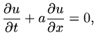
Example 2: Lax-Wendroff applied to a hyperbolic equation

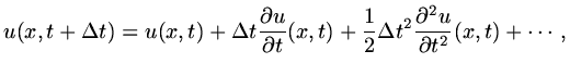
One important method to generate a finite difference scheme is Lax-Wendroff whereby the time derivatives in a Taylor expansion of $u(.,t+\Delta t )$ about $t$ are replaced by space derivatives using the differential equation, and those space derivatives discretised using finite differences. We consider the model equation

$${{\partial u}\over{\partial t}}+a{{\partial u}\over{\partial x}}=0,$$ (108)

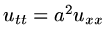
where $a$ is constant. Since

$$u(x,t+\Delta t)=u(x,t)+\Delta t {{\partial u}\over{\partial t}}(x,t)+{1\over 2}\Delta t^2{{\partial^2 u}\over{\partial t^2}}(x,t)+\cdots ,$$ (109)

and using $u_t=-au_x$, $u_{tt}=a^2u_{xx}$,

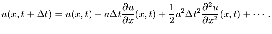$$u(x,t+\Delta t)=u(x,t)-a\Delta t{{\partial u}\over{\partial x}}(x,t)+{1\over 2}a^2\Delta t^2{{\partial^2 u}\over{\partial x^2}}(x,t)+\cdots .$$ (110)

This series is truncated after the third term to give a second order accurate scheme,

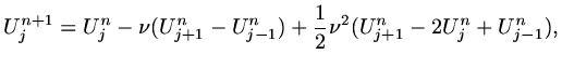$$U^{n+1}_j=U^n_j-\nu (U^n_{j+1}-U^n_{j-1})+{1\over 2}\nu^2 (U^n_{j+1}-2U^n_j+U^n_{j-1}),$$ (111)

where $\nu=a\Delta t/h$. Substituting a Fourier mode gives,

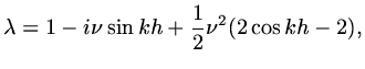$$\lambda =1-i\nu\sin kh+{1\over 2}\nu^2(2\cos kh-2),$$ (112)

so that $\lambda$ is complex. If $p=\sin{1\over 2}kh$,

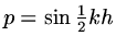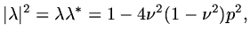$$\vert\lambda\vert^2=\lambda\lambda^*=1-4\nu^2(1-\nu^2)p^2,$$ (113)

and we will have $\vert\lambda\vert\le 1$ provided $-1\le \nu\le 1$.

Example 3: $\theta$-method for Diffusion Equation

If we apply a $\theta$-method to a diffusion equation, then

$$U^{n+1}_j-\mu\theta (U^{n+1}_{j+1}-2U^{n+1}_j+U^{n+1}_{j-1})= U^n_j+\mu (1-\theta )(U^n_{j+1}-2U^n_j+U^n_{j-1}),$$ (114)

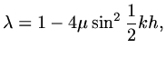
where again $\mu=D\Delta t/h^2$. Substituting in a Fourier mode,

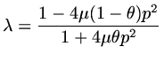$$\lambda={{1-4\mu (1-\theta )p^2}\over{1+4\mu\theta p^2}}$$ (115)

with $p=\sin{1\over 2}kh$. We deduce that $\vert\lambda\vert\le 1$ provided

$$\theta\ge {1\over 2}-{1\over{4\mu}}.$$ (116)