chapter9

(i) We have noted that two-dimensional composite expansions have been little used. Can you firstly use the suggested composite expansion to generate the stream-function through a channel and contour lines of constant $\psi$ ? Can you develop an improved two-dimensional composite expansion?

(ii) One of the unsatisfactory features of predictions for channel flow is that of separation on both walls which comes from the $\epsilon=o(R^{-1/7})$ theory of chapter 8. We have shown one example where allowance of a cross channel pressure gradient results in separation being absent from the solution on the opposite flat wall in Figure 9.7. If we try to compute the equivalent flow for the channel with lower wall defined by (8.103) but allowing the pressure to vary across the channel then the computation is fraught with difficulty. Convergence is extremely slow and may be affected by an instability which develops as the number of iterations increases. 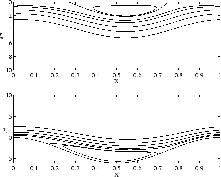An example of a flow calculated after 150 iterations using 51 mesh points in the

-direction and

across each boundary layer (so that a $609\times 609$ matrix has to be inverted each Newton step) is shown in Figure 0.1. The separation region on the flat wall is still evident although it has moved slightly downstream relative to that in the furrowed wall.

**Figure **Fig. 0.1**:** Solution of two layer interactive equations for $\mu = 6.08$ after 150 iterations.
$\begin{figure}\centerline{\psfig{file=newdeck2.50x100.psi2.eps,width=4.in}}\end{figure}$

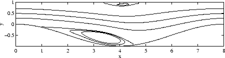
If we look at computation or observation of steady flow, separation on the opposite wall is not usually present. However, separation on the opposite flat wall is observed, see Sobey(1985) Figure 8 (a)), and can be computed, see Figure 0.2, during the acceleration phase of unsteady flow. Were the observations to only be during the deceleration phase then the extra adverse pressure gradient from the deceleration could aid the occurrence of separation but these observations and calculations are for flows which have been accelerating. Is there any relation between the prediction from steady theory of separation on the flat wall and the unsteady solutions. Does the extra acceleration of the fluid result in the fluid behaving as if it were at a much greater Reynolds number? To complicate matters the calculation of separation on the flat wall during an acceleration does not happen for all Strouhal numbers, there seems to be a band on values, greater than quasi-steady flow but not so large that viscous effects dominate for which this second vortex can be computed.

Are there a number of artificial effects happening in the interactive boundary layer computations: are the computations properly mesh converged, are they properly converged for a fixed mesh, is the simple method used to solve the interactive equations inadequate to resolve these questions and a more sophisticated method (for instance a spectral method) more appropriate for computing solutions to the interactive equations when applied to periodically varying channels?

**Figure **Fig. 0.2**:** Computed solution of unsteady Navier-Stokes equations at instant of peak flow, for oscillatory flux.
$\begin{figure}\centerline{\psfig{file=long001c.r300.s03.t25.psi.eps,width=4.in}}\end{figure}$

(i) deck2.f `triple deck' solution allowing cross channel pressure variation
(ii) freeint.f free interaction development of separation in a parallel channel