


Next: 2 Conjugate Gradient Iteration
Up: 1 Introduction
Previous: 4 Some General Theory
Contents
Consider now the discretisation of
![$\displaystyle \nabla^2 w=f,\ \ (x,y)\in [0,1]\times [0,1]$](img395.png) |
(157) |
with condition  on the boundary. If we use central differences with mesh size
 in both
  and
and  directions,
 |
(158) |
and boundary conditions
 ,
,
 and
and
 . For an appropriately defined vector
 we have
 |
(159) |
 |
(160) |
Suppose that  is an eigenvalue of the Jacobi iteration matrix for this problem,
then
is an eigenvalue of the Jacobi iteration matrix for this problem,
then
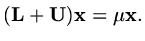 |
(161) |
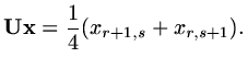
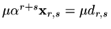
Consider now a vector
 whose elements are defined by
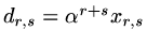 ,
then the
,
then the
 element of
 is
is
 |
(162) |
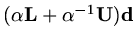
and the RHS is
 so that is also an
eigenvalue of the matrix
so that is also an
eigenvalue of the matrix
 for any
  .
.

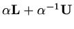
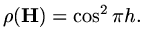
If we define the asymptotic convergence rate as  the Lemma implies that
Gauss-Seidel converges twice as fast as Jacobi. To show this result in this case (it is a more
general result valid for a wider class of matrices) we use the fact that
the Lemma implies that
Gauss-Seidel converges twice as fast as Jacobi. To show this result in this case (it is a more
general result valid for a wider class of matrices) we use the fact that
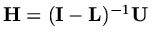
 so that
![$\displaystyle {\rm det}(\lambda{\rm\bf I}-{\rm\bf H})={\rm det}[({\rm\bf I}-{\r...
...m\bf I}-{\rm\bf H})]={\rm det}[\lambda{\rm\bf I}-\lambda{\rm\bf L}-{\rm\bf U}],$](img418.png) |
(163) |
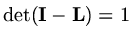
since
 , so that
![$\displaystyle {\rm det}(\lambda{\rm\bf I}-{\rm\bf H})= {\rm det}[\sqrt{\lambda}...
...mbda}{\rm\bf I}-\sqrt{\lambda}{\rm\bf L}-{1\over\sqrt{\lambda}}{\rm\bf U})]=0,,$](img420.png) |
(164) |
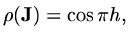
and using our result above,
 must be an eigenvalue of
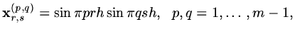
In addition to this result we can find the eigenvalues and eigenvectors of
 explicitly.
If we let
explicitly.
If we let
 |
(165) |
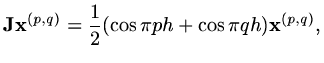
then
 |
(166) |
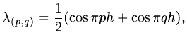
and the eigenvalue associated with eigenvector
 is
is
 |
(167) |
so that the largest eigenvalue occurs when  or
or  and
and
 |
(168) |
 |
(169) |
Next: 2 Conjugate Gradient Iteration
Up: 1 Introduction
Previous: 4 Some General Theory
Contents
Last changed 2000-11-21