


Next: 2 Finite Volume Methods
Up: 1 Model Problem
Previous: 1 Model Problem
Contents
Subsections
The definition of derivative can be used to obtain a discrete
approximation, since the definition can be expressed in a number
of different ways, so to can the discrete approximation. The definition
in terms of limits can be any of
 |
(7) |
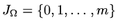
Define a set of points
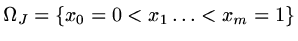 and a set of nodes
 and approximate
 by
by  ,
,
 .
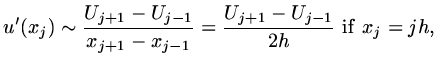
Then discrete approximations for a derivative are:
.
Then discrete approximations for a derivative are:
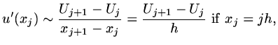 |
(8) |
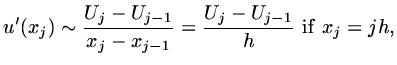 |
(9) |
 |
(10) |
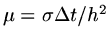
For simplicity take  with
with  unless it is indicated otherwise.
Higher derivatives can be approximated in a similar way:
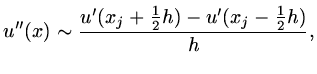 |
(11) |
so that
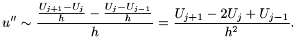 |
(12) |
Now if
 ,
,  and
and  ,
,
 |
(13) |
 |
(14) |
 |
(15) |
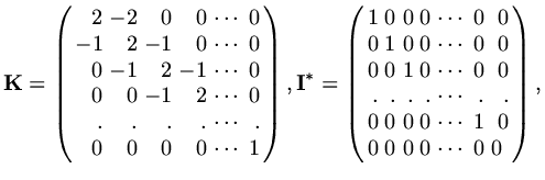
If we let
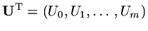 be a vector of approximate values,
define matrices
be a vector of approximate values,
define matrices
 ,
,
 ,
,
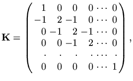 |
(16) |
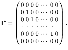 |
(17) |
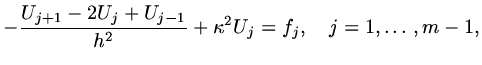
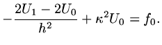
Then we can write the finite difference scheme as
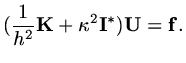 |
(18) |
This is a discrete version of the original differential equation (1.6).
It is possible to reduce the matrices to
 by eliminating
the explicitly given values of
by eliminating
the explicitly given values of  ,
,  . On the other hand, if one of the boundary
conditions involved a derivative (corresponding to a physical situation where
as an example, heat transfer rate is specified) then keeping these values as "unkowns"
is needed; overall keeping them in the matrix is a very small overhead.
. On the other hand, if one of the boundary
conditions involved a derivative (corresponding to a physical situation where
as an example, heat transfer rate is specified) then keeping these values as "unkowns"
is needed; overall keeping them in the matrix is a very small overhead.
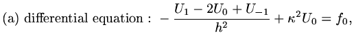
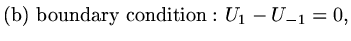
If the boundary condition at  is for instance
  we proceed by
introducing a fictitious point
we proceed by
introducing a fictitious point  , so that we have
 |
(19) |
 |
(20) |
and eliminating ,
 |
(21) |
,
become
 |
(22) |
If the problem is unsteady, for instance
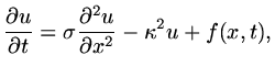 |
(23) |
then introduce a set of time points
 (usually assuming
 )
and let
)
and let  approximate
 . Than approximate
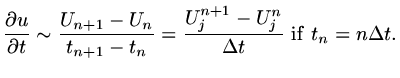 |
(24) |
It is now possible to use a variety of schemes.
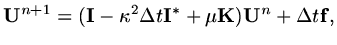
(a) Explicit Scheme
If we approximate the RHS of the differential equation at time  , and
let
, and
let
 and define a vector
 at each time step,
 |
(25) |
the vector  is given explicitly in terms of known quantities so there is no
matrix problem to solve.
is given explicitly in terms of known quantities so there is no
matrix problem to solve.
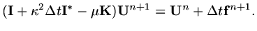
(b) Implicit Scheme
Approximate the RHS of the differential equation at
time  ,
,
 |
(26) |
Now a matrix problem has to be solved at each time step.
(c)  -method
We approximate the right hand side as a weighted sum of values at and ,
using
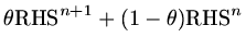 ,
,
![$\displaystyle [{\rm\bf I}+\theta \kappa^2\Delta t {\rm\bf I}^*-\theta\mu{\rm\bf...
...ta)\mu{\rm\bf K}]{\rm\bf U}^n +\theta {\rm\bf f}^{n+1}+(1-\theta ){\rm\bf f}^n.$](img68.png) |
(27) |
The case
 is called Crank-Nicholson and has a higher order of accuracy
in approximating the time derivative than the other cases (see note 4 below).
is called Crank-Nicholson and has a higher order of accuracy
in approximating the time derivative than the other cases (see note 4 below).
If steady but two-dimensional, for instance
![$\displaystyle -\nabla^2 u+\kappa^2u=f\ \ {\rm on}\ \Omega=[0,1]\times [0,1],$](img70.png) |
(28) |
let  approximate
 ,
,
 ,
,
 where
where
 ,
,
 , and approximate
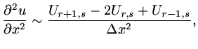 |
(29) |
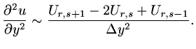 |
(30) |
The discrete form of the differential equation is
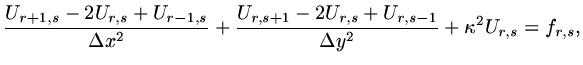 |
(31) |
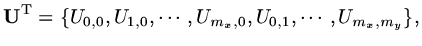
Now we need to define the vector
 to include all the elements of the
array . One way is just to enumerate the elements of
,
to include all the elements of the
array . One way is just to enumerate the elements of
,
 |
(32) |
another is to suppose there is a map
 which maps the pairs
  to
the integers
to
the integers
 .
Either way,
is a vector of dimension
.
Either way,
is a vector of dimension
 - a partial explanation
of why supercomputers are needed for anything like realistic problems. Even using
only
- a partial explanation
of why supercomputers are needed for anything like realistic problems. Even using
only
 points means we have to determine a vector of length
  by inverting a matrix system where the coefficient matrix is
roughly of size
by inverting a matrix system where the coefficient matrix is
roughly of size
 .
If we now define one row of a matrix
by
.
If we now define one row of a matrix
by
 |
(33) |
with
suitably defined, we still have a matrix system
 |
(34) |
to invert in order to calculate
. In a later part we shall consider
algorithms which can invert matrix systems such as this where it is impossible
to store the whole coefficent matrix on a computer; all we are able to store is the vector
obtained when the matrix multiplies another vector.
If we write the continuous system as
 |
(35) |
and the discrete system as
 |
(36) |
where
 ,
,  are linear operators,
then define a truncation error
are linear operators,
then define a truncation error
 |
(37) |
and an error
 |
(38) |
We then have
 |
(39) |
This is a central result in analysis of errors associated with discretisation.
In principle, to determine the magnitude of errors, we have only to know the `magnitude'
(that is some form of norm)
of the inverse of and the `magnitude' of the truncation error.
In our model problem
 |
(40) |
so that
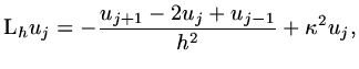 |
(41) |
and using Taylor expansions,
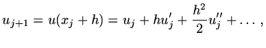 |
(42) |
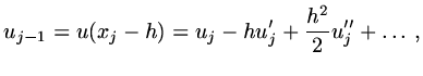 |
(43) |
and hence
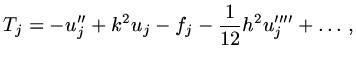 |
(44) |
the first three terms are just the differential equation evaluated at  and so add to zero; with a bit more work, we can show
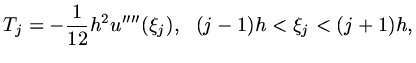 |
(45) |
so that if
 , then
 |
(46) |
If  as
as  the scheme is called consistent.
If  as the scheme is called order-
 accurate. In the model
problem, the scheme is second order accurate. With PDE's, it is possible for the accuracy to
be of different order for different independent variables. In the problem considered in
note 2 above, the scheme is second order accurate in
accurate. In the model
problem, the scheme is second order accurate. With PDE's, it is possible for the accuracy to
be of different order for different independent variables. In the problem considered in
note 2 above, the scheme is second order accurate in  but only first order accurate
in
but only first order accurate
in  , unless using crank-Nicholson when it is second order accurate
in .
, unless using crank-Nicholson when it is second order accurate
in .
If we define
 ,
,
 , then in matrix notation
 |
(47) |
and formally
 |
(48) |
so we need an estimate of the norm of
 . This turns out to be
 in our model problem so that
 as .
as .
Next: 2 Finite Volume Methods
Up: 1 Model Problem
Previous: 1 Model Problem
Contents
Last changed 2000-11-21