


Next: 2 Stability
Up: 1 Model Problem
Previous: 2 Finite Volume Methods
Contents
Subsections
The finite element method has now quite a long and interesting history. It was
originally developed by engineers dealing with structural analysis. They realised that
if say a loaded plate was divided into small triangles or quadrilaterals (`elements')
and the displacement within an element was assumed to be linear in space variables, then
the stress could be calculated throughout the element and the sum of all the stresses
would have to agree with the loading. Hence they obtained a linear combination of
displacements equal to the loading, and inverting this system gave the displacements
and then the stresses in the structure. It was quickly realised that this very
practical method could be put in a sound mathematical framework, and once that
framework was
developed, the method could be applied to problems other than structural analysis. We shall
look only at the modern understanding of finite elements. It is important to
distinguish our understanding of how finite element analysis approximates
the solution of a differential system from the details of how the method is implemented.
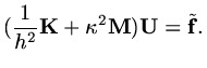
We seek a solution of
 on
on
 and its associated boundary
conditions. In finite
differences we tried to find a set of values {
and its associated boundary
conditions. In finite
differences we tried to find a set of values { } which approximated
  at a set of
points in the domain. Now ask the question. Suppose we have a set of simple
functions, can we approximate using these functions? In abstract terms,
if
at a set of
points in the domain. Now ask the question. Suppose we have a set of simple
functions, can we approximate using these functions? In abstract terms,
if
 and we have a set of (possibly) simple functions
 can we find a function
 which is a good
approximation to ? Obviously this immediately points us towards needing some
way of measuring how good one function represents another: that is we need some way
of measuring distance in the set of functions
which is a good
approximation to ? Obviously this immediately points us towards needing some
way of measuring how good one function represents another: that is we need some way
of measuring distance in the set of functions
 . One way to achieve this
is to use an inner product, for instance if
. One way to achieve this
is to use an inner product, for instance if  we can define
 |
(55) |
to be an inner product and then we can measure the size of a function by
 |
(56) |
and `distance' between functions by
 |
(57) |
The definition of `distance' is not unique, for the inner product example, the weight function
 will affect the calculation of `distance'.
The approximation problem can now be posed very precisely: Given
and a subset
can we find
such that
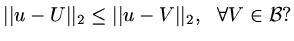 |
(58) |
In the case of a norm based on an inner product we can go someway to answering this
question.
Since
 |
(59) |
we have
 |
(60) |
Since the last term could be positive or negative, whereas the second last term is
alsways positive, in order for
 |
(61) |
we need only
 |
(62) |
This is now called Galerkin orthogonality. It is just a generalisation of our physical
intuition that in coordinate geometry, if you wanted the point on a straight line
closest to a curve, you would make the line from the approximating point on the
straight line to the curve perpendicular to the straight line.
Before we finally deal with the finite element method we need to re-look at the
differential equation. We have already seen that many systems come from conservation
laws which deal with integrals over volumes of quantities. We have also seen that
in the finite volume method, we reversed this by looking at an integral of the
equation over a small `volume'. Now we generalise this further by saying that instead
of requiring
 , for some set of functions
 we require the inner product of the equation with all functions in this
space to be zero:
we require the inner product of the equation with all functions in this
space to be zero:
 |
(63) |
This is usually called a weak form of the equation.
One reason for doing this is that we can try to use integration by parts
to reduce the highest derivative of which occurs. Another reason is that many
conservation laws have solutions which give an extremum of some functional and these
very natuarlly fall into this framework.
In the case of our model problem, a solution of the differential equation
needs to be twice differentiable. If we can integrate by parts we need only consider
functions which have integrable derivatives (so the derivative does not need to be
continuous). There are special symbols for this space of functions and some of its
subspaces.
![$\displaystyle H^1[0,1]=\{{\rm functions\ }u{\rm\ on\ }[0,1]{\rm\ with\ } \int_0^1({u'}^2+u^2){\rm d}x\ {\rm bounded},$](img151.png) |
(64) |
We will usually just write  and leave the domain ambiguous.
 |
(65) |
 |
(66) |
The weak form of our equation is
 |
(67) |
and if we integrate by parts
 |
(68) |
The variational form of the equation is: find
 such that
![$\displaystyle J[u]=\int_0^1[{1\over 2}({u'}^2+\kappa^2u^2)-fu]{\rm d}x,$](img158.png) |
(69) |
is an extremum. We shall not take this further here.
If we define a new inner product:
 |
(70) |
this can be used to define a new norm, sometimes called an energy norm,
 |
(71) |
and the weak form of the equation is
 |
(72) |
This has now established the framework within which we can apply finite elements.
Instead of looking for the solution of a differential equation, we are seeking a
function
(as it is in  it automatically satisfies the boundary conditions)
which satisfies the weak form, an integral equation, for all functions in
it automatically satisfies the boundary conditions)
which satisfies the weak form, an integral equation, for all functions in  .
.
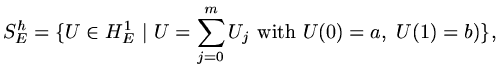
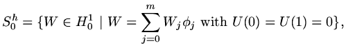
We now wish to approximate the function throughout the whole interval, ![$ [0,1]$](img164.png) ,
on which it is defined. It is logical to look at functions which are already in ,
for instance we might choose functions which are piecewise linear. In the
background, but not
needed to be specified at this point, is that there is a mesh (or set of elements)
which cover the interval and they have some characteristic size, say
,
on which it is defined. It is logical to look at functions which are already in ,
for instance we might choose functions which are piecewise linear. In the
background, but not
needed to be specified at this point, is that there is a mesh (or set of elements)
which cover the interval and they have some characteristic size, say  . For instance
the simplest set of elements would come from dividing the interval by the set of points
. For instance
the simplest set of elements would come from dividing the interval by the set of points
 where
where  so that the elements are the
intervals
so that the elements are the
intervals
![$ [jh,(j+1)h],\ j=0,\ldots ,m-1$](img166.png) . Suppose we have chosen a set of approximating
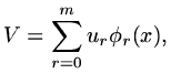
functions in and we let
. Suppose we have chosen a set of approximating
functions in and we let
 |
(73) |
 |
(74) |
We see that
 , and
, and
 .
.
Now
 will be a best approximation to
measured in the
will be a best approximation to
measured in the  -norm if the error is orthogonal (orthogonality measured using the -inner product)
to all functions in
-norm if the error is orthogonal (orthogonality measured using the -inner product)
to all functions in  ,
,
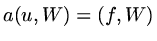
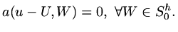 |
(75) |
Now  is a linear operator and we know that the weak form which satisfies
gives that as
is a linear operator and we know that the weak form which satisfies
gives that as
 then
then
 , so that the orthogonality
condition is
, so that the orthogonality
condition is
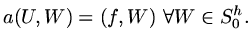 |
(76) |
This is the essence of the finite element method: if we can find  then it is
a best approximation to measured in a particular norm (in this case the -norm).
then it is
a best approximation to measured in a particular norm (in this case the -norm).
To make this useful we have to carry on a bit to understand how we can calculate .
We suppose that we use a set of linearly independent basis functions
 (linear independence measured using the inner product) such that
 |
(77) |
 |
(78) |
then since is a linear subspace the condition which determines can also
be written
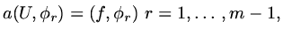 |
(79) |
and if we substitute the form of in terms of the basis funcitons,
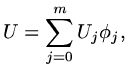 |
(80) |
then
 |
(81) |
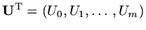
This is just a matrix equation for the vector
 (it is incomplete, it needs the addition of the two boundary conditions to produce a
full matrix). This is still a very general framework so we now focus on one example
implementation of this finite element framework.
(it is incomplete, it needs the addition of the two boundary conditions to produce a
full matrix). This is still a very general framework so we now focus on one example
implementation of this finite element framework.
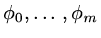
Suppose the functions  are piecewise linear functions,
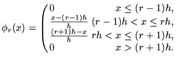 |
(82) |
We next need to evaluate the numbers
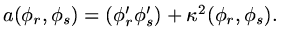
(a)
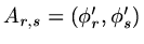
If  or
or  then
then  , if
, if  or
or  ,
,
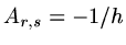 ,
if
,
if  ,
,
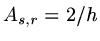 .
.
(b)
 If or then
  , if or ,
 ,
if ,
,
if ,
 .
.
if we define
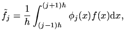 |
(83) |
then we must have
 |
(84) |
if we define a `mass' matrix
 by
by
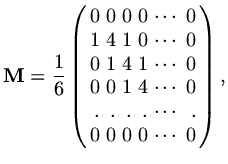 |
(85) |
and use the same matrix
 as occured in finite difference and finite volume formulations, then in our model problem the vector
 is determined by
 |
(86) |
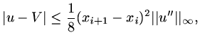
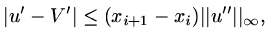
We are not able to go into error analysis of finite element methods in great detail.
There are very readable sections in Eriksson et al which you are advised to read through.
One key idea is as follows: since we have a best approximation (measured in the energy norm)
the error in that norm must be bounded by the error which occurs for any other approximating
function, so we choose an interpolating approximation since Lagrange's theorem tells us the
error in interpolating functions.
Mathematically, since
 |
(87) |
using the same piecewise linear functions , choose
 |
(88) |
and Lagrange's theorem gives
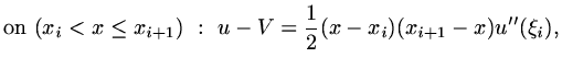 |
(89) |
where
 so that
 |
(90) |
and similarly
 |
(91) |
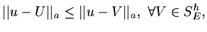
so we have a a priori error estimate
![$\displaystyle \vert\vert u-U\vert\vert_a^2\le [h^2+{1\over{64}}\kappa^2h^4]\vert\vert u''\vert\vert_\infty.$](img213.png) |
(92) |
This may appear a little weak, since it indicates an error in the energy norm which
is only first order in , but with more analysis better error estimates can be found.
Once we have an approximate solution  , one sensible question is `how well
does satisfy the original differential equation?' Of course this needs to
be carefully thought out because there will be a set of points (the boundaries of elements)
where cannot be differentiated sufficiently to be substituted into the equation.
As this is ony a finite set of points, we can still calculate integrals across
the domain.
, one sensible question is `how well
does satisfy the original differential equation?' Of course this needs to
be carefully thought out because there will be a set of points (the boundaries of elements)
where cannot be differentiated sufficiently to be substituted into the equation.
As this is ony a finite set of points, we can still calculate integrals across
the domain.
We start by defining a residual function
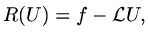 |
(93) |
on each interval
 and a mesh function
  by
by
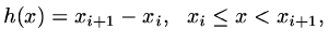 |
(94) |
so with a uniform mesh, is just a constant but with a variable mesh, gives the
local mesh size.
Intuitively, a measure of how well the approximation represents the solution
is given by an integral of the residual across the domain, so if the residual
is relatively large we should think of changing the mesh to reduce the residual,
if the residual is relatively small, the mesh could be expanded.
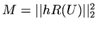
We cannot go into the mathematics too deeply, but it is possible to derive results
for our model problem of the form
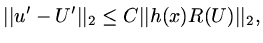 |
(95) |
for some positive constant  .
This means we can produce an algorithm to adapt the mesh to a particular
problem and to achieve a given tolerance for some measure of the error.
In this case we can seek to make
.
This means we can produce an algorithm to adapt the mesh to a particular
problem and to achieve a given tolerance for some measure of the error.
In this case we can seek to make
 less than some tolerance
by firstly moving mesh points, and then increasing the number of mesh points.
less than some tolerance
by firstly moving mesh points, and then increasing the number of mesh points.
As an example, consider the case  and approximation using piecewise linear functions,
when the residual is just
and approximation using piecewise linear functions,
when the residual is just  ,
and we take
,
and we take
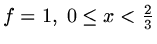 ,
,
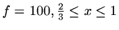 .
If we take four points uniformly across the interval, then
.
If we take four points uniformly across the interval, then  .
If however we move the mesh so the four points are at
.
If however we move the mesh so the four points are at
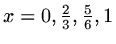 ,
then
,
then  and if we add one more point, so the points are
at
and if we add one more point, so the points are
at
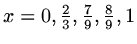 then
then  .
If five points were to be uniformly distributed across
the interval them
.
If five points were to be uniformly distributed across
the interval them  . Since such large gains can be made using an
algorithmic approach, mesh adaptation is becoming more important in the numerical
solution of PDE's.
. Since such large gains can be made using an
algorithmic approach, mesh adaptation is becoming more important in the numerical
solution of PDE's.
Next: 2 Stability
Up: 1 Model Problem
Previous: 2 Finite Volume Methods
Contents
Last changed 2000-11-21